Anomaly Detection

Written on 2014-07-10

Definition of Time Series

Definition $\def\KM{\mathcal{M}} \def\IY{\mathbb{Y}}$

A time series (instance) $y$ is a sequence of real numbers:

$y = (y_1, \dots, y_T)$

A time series model $\IY$ is a sequence of random variables:

$\IY = (\IY_1, \dots, \IY_T)$

Examples $\def\eps{\epsilon}$ $\def\KN{\mathcal{N}}$ $\def\IR{\mathbb{R}}$

Let $\eps_t \sim \KN(0,1)$ be independent standard-normally distributed. Then the time series model with $\IY_t = \eps_t$ is called standard-white noise.
Let $b \in \IR$ be a real number, then $\IY_t = b + \eps_t$ is a time series model with constant expectation $E[\IY_t] = b$
Let $b,m \in \IR$ be real numbers, then $\IY_t = b + m t + \eps_t$ is a time series with affine-linear expectations $E[\IY_t] = b + m t$

Remark

For a given time series $y$ and model $\IY$ we get a probability for the occurencye of $y$ :

$P_{\IY}[y] = P[\IY_1 = y_1, \dots, \IY_T = y_T].$

In case the model has a joint probability density function $p_\IY$ we get a probability density for the time series $y$ :

$p_{\IY}(y) = p_{\IY_1, \dots \IY_T}(y_1, \dots, y_T)$

## Numerical Simulation of Examples

import random
from matplotlib import pyplot as plt
plt.rcParams['figure.figsize'] = (9.0, 3.0)

eps = lambda : random.normalvariate(0,1)

Y1 = [ eps() for i in range(100)]
Y2 = [ eps() + 5 for i in range(100)]
Y3 = [ eps() - 3 + 0.2 * i for i in range(100) ]

plt.title("Time series samples")
plt.plot(Y1, 'r.', label="Standard white noise")
plt.plot(Y2, 'g.', label="Normal noise with mean")
plt.plot(Y3, 'b.', label="Normal noise with mean and drift")
plt.legend(loc = "upper left")
plt.show()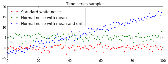

png

Parameter Estimation

Definition Let $\IY_\theta$ for $\theta \in \Theta$ be a family of time series models, and let $y$ be a time series instance. We write $P_\theta$ and $p_\theta$ for $P_{\IY_\theta}$ and $p_{\IY_\theta}$ .

The maximum likelihood estimator (MLE) (cf. wikipedia) for $y$ in $\Theta$ is defined as

$\hat{\theta}= \text{arg-max} \{ P_\theta[y] \,\vert\, \theta \in \Theta \}.$

In case the model has a density function $p$ we set

$\hat{\theta}= \text{arg-max} \{ p_\theta[y] \,\vert\, \theta \in \Theta \}.$

Note that the maximum likelyhood estimater does not need to exists, nor is it unique if it exists.

Example

Let $\Theta=\IR$ and $\theta = b$ with model $\IY_t = b + \eps_t$ , then

$p_b(y) = \frac{1}{2 \pi} exp(-\frac{1}{2} \sum_t (y_t - b)^2 ).$

The value $p_b$ is maximal if the sum of squares $\sum_t (b - y_t)^2$ is mininmal. Threfore

$\hat{b} = \frac{1}{T} \sum y_t.$

Similarly, for the model $\IY_t = b + m t + \eps$ and $\theta=(b,m)$ the MLE minimizes the following sum of squares

$\sum_t (b + m t - y_t)^2.$

This problem is quivalent to Linear Regression.

# Linear Regression Example adapted from
# http://glowingpython.blogspot.de/2012/03/linear-regression-with-numpy.html

import numpy as np
from scipy import stats

y = [19, 20, 20.5, 21.5, 22, 23, 23, 25.5, 24]
T = np.arange(0,9)

m, b, _,_,_ = stats.linregress(T,y)

line  = b + m * T
const = np.mean(y) + 0 * T

plt.title("MLE Estimators")
plt.plot(T,y,'ro', T, const, 'g-', T,line,'b-')
plt.legend(("Samples", "Mean", "Regression line"), loc="upper left")
plt.show()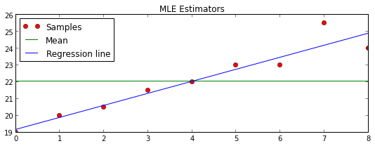

png

Hypothesis Testing

Let $\IY_\theta$ and $\IY_{\theta'}$ be two families of models, indexed by $\theta \in \Theta_0, \theta' \in \Theta_1$ and $y$ a time series instance. We consider the following statements:

$H_0:$ The sample $y$ was drawn from a model in $\{\IY_\theta\}$
$H_1:$ The sample $y$ was drawn from a model in $\{\IY_{\theta'} \}$

In order to decide between those statements, we consider their likelihood ratio.

Definition

We define the Likelihood ratio $\Lambda$ to be

$\Lambda = \frac{max \{ P_{\theta'}[y] \,\vert\, \theta' \in \Theta_1 \}}{max \{ P_{\theta}[y] \,\vert\, \theta \in \Theta_0 \} } = \frac{ P_\hat{\theta'}[y] }{ P_\hat{\theta}[y]}$

or, in the continues case

$\Lambda = \frac{max \{ p_{\theta'}[y] \,\vert\, \theta' \in \Theta_1 \}}{max \{ p_{\theta}[y] \,\vert\, \theta \in \Theta_0 \} } = \frac{p_\hat{\theta'}[y] }{ p_\hat{\theta}[y]}$

We define the Log-likelihood ratio as $\lambda = log(\Lambda)$ .

For a given confidence level $\alpha \geq 1$ we accept the Hypythesis $H_1$ if $\Lambda > \alpha$ .

Example $\def\half{\frac{1}{2}}$

Take $b_0 < b_1 \in \IR$ , a time series $y$ and $\theta = b_0, \theta' = b_1$ . To test the hypothesis

$H_0$ : The instance $y$ was drawn from $\IY_t = b_0 + \eps_t$
$H_1$ : The instance $y$ was drawn from $\IY_t = b_1 + \eps_t$

we calculate the likelihood ratios as:

$\begin{align} \lambda &= log(\frac{ 1 / \sqrt{2 \pi} exp(-\half \sum_t (y_t - b_1)^2 )}{ 1 / \sqrt{2 \pi} exp( - \half \sum_t (y_t - b_0)^2)}) \\ &= \half \sum_t (y_t - b_0)^2 - (y_t - b_1)^2 \\ &= \half \sum_t (y_t - \bar{b} + \delta)^2 - (y_t - \bar{b} - \delta)^2 \\ &= 2 \delta \sum_t (y_t - \bar{b}) \\ &= 2 \delta T (\bar{y} - \bar{b}) \end{align}$

where $\bar{b} = \half (b_0 + b_1)$ is the average of $b_0, b_1$ , the variable $\delta = \half(b_1 - b_0)$ is half the distance between $b_1$ and $b_0$ and $\bar{y} = \frac{1}{T} \sum_t y_t$ is the sample mean. For the second step we used the following simple identity:

$(a + b)^2 - (a - b)^2 = 4ab$

Note, that $\lambda = 0$ if $\bar{b} = \bar{y}$ . And $\lambda > 0$ if $\bar{y} - \bar{b} > 0$ , i.e. $\bar{y}$ is closer to $b_1$ than to $b_0$ .

We accept the Hypothesis $H_1$ if $\lambda > log(\alpha)$ , which is equivalent to:

$\bar{y} - \bar{b} > \frac{log(\alpha)}{2 \delta T}$

# Numerical Hypothesis Test Example

from scipy.stats import norm

# Model Parameters
b0 = 0
b1 = 5
alpha = 10

def normal_density(b):
    return lambda y : norm.pdf(loc=b,scale=1,x=y)

# probability density functions
p0 = normal_density(b0)
p1 = normal_density(b1)

plt.title("Probability Density Functions")
grid = np.linspace(-5,10,100)
plt.plot(grid,map(p0, grid))
plt.plot(grid,map(p1, grid))
plt.show()

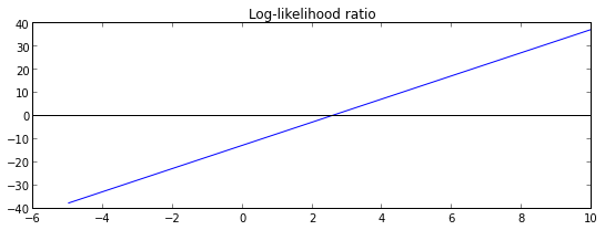
# Log likelihood ratio (for single sample)
l = lambda y : np.log(p1(y) / p0(y))
plt.plot(grid,map(l, grid))
plt.title("Log-likelihood ratio")
plt.axhline(color = 'black')
plt.show()

b     = 1. / 2 * (b0 + b1)
delta = 1. / 2 * (b1 - b0)

l2 = lambda x : 2*delta*(x - b)

print "l2 == l ? " + str(np.max(map(lambda x: l(x) - l2(x), grid)) < 10**-7)

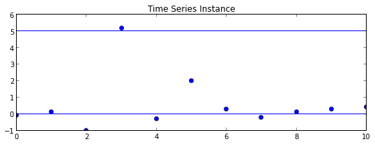
# Time series instance
Y = [0.1,0.3,.4,.1,-.1,-0.3,0.3,-0.2,2,-1,5.2]*1
random.shuffle(Y)

plt.title("Time Series Instance")
plt.plot(Y, 'o')
plt.axhline(b0)
plt.axhline(b1)
plt.show()

log_lhr = lambda Y : sum(l2(y) for y in Y)

from IPython.display import Latex

print "Hypothesis H_1 accepted: {}".format(log_lhr(Y) > np.log(alpha))
Latex("Log likelihood ratio $$\lambda={}$$ for plotted time series Y".format(log_lhr(Y)))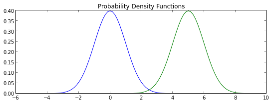

png

l2 == l ? True

png

Hypothesis H_1 accepted: False

Log likelihood ratio $\lambda=-103.5$ for plotted time series Y

Test for changes in mean

For given $b_0 < b_1$ we consider the hypotheses:

$H_0$ : Constant mean model $\IY_t = b_0 + \eps_t$
$H_1$ : Change in mean at a time $k \in \{ 0, \dots, T\}$ : $\IY_t = b_0 + \eps_t, \text{ for } t \leq k$ $\IY_t = b_1 + \eps_t, \text{ for } t > k$

For an instance $y$ we calculate the log-likelihood ration to be $\lambda = \max_k \{ \lambda_k \}$ and using the notation from the last example we get

$\begin{align} \lambda_k &= \half [ \sum_t (y_t - b_0)^2 - \sum_{t \leq k} (y_t - b_0)^2 - \sum_{t > k} (y_t - b_1)^2 ] \\ &= \half \sum_{t > k} (y_t - b_0)^2 - (y_t - b_1)^2 \\ &= 2 \delta \sum_{t > k} (y_t - \bar{b}) \end{align}$

We introduce the notation $S_k^l = 2 \delta \sum_{t=k}^l (y_t - \bar{b})$ so that we can write

$\lambda_k = S_{k+1}^T = S_1^T - S_1^k$

The total log likelihood ratio is computed by explicit maximization:

$\lambda = \max_k \{ \lambda_k \} = S_1^T - \min_k \{ S_1^k \}$

Note, that $\lambda \geq 0$ , since $\min \leq S_1^T$ .

log_lhr_k = lambda k, Y : 2 * delta * sum(y - b for y in Y[k+1:])
log_lhr_max = lambda Y : max( log_lhr_k(k,Y) for k in range(len(Y)))

Y = [0.1,0.3,.4,.1,-.1,-0.3,0.3,-0.2,2,-1,5.2,5,6,7,4,5]

ax = plt.axes()
ax.set_title("Time Series, Model-expectations and log-likelihood ratio")
ax.plot(Y, 'o')
ax.axhline(b0)
ax.axhline(b1)
ax2 = ax.twinx()
ax2.plot([log_lhr_k(k,Y) for k in range(len(Y))], 'y--')

plt.show()

Latex("$$\lambda = \max \lambda_k = {} $$".format(log_lhr_max(Y)))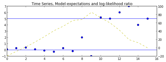

png

$\lambda = \max \lambda_k = 86.0$

Online Variant

It turns out, that there is a simple recursion, which allows us to compute the likelyhood ratio $\lambda(T+1)$ for an instance $y_1,\dots,y_T$ of length $T+1$ from the knowledge of $\lambda(T)$ for the instance $(y_1,\dots,y_T)$ of length $T$ .

Indeed, we have $\lambda(T+1) = S_1^{T+1} - \min_{k=1,\dots,T+1} S_1^{k}.$ Note, that $S_1^{T+1} = S_1^T + 2 \delta (y_t - \bar{b})$ .

The minimum-term we have

$\quad \min_{k=1,\dots,T+1} S_1^{k} = \begin{cases} S_1^{T+1} && (A)\\ \min_{k=1,\dots,T} S_1^{k} && (B) \end{cases}.$ In case $(A)$ we have $\lambda(T+1) = 0$ and in case $(B):$ $\lambda(T+1) = \lambda(T) + 2 \delta (y_{T+1} - \bar{b}).$

Since we always have $\lambda(T) \geq 0$ , we get the total recursion:

$\lambda(T + 1) = \max \{ 0, \lambda(T) + 2 \delta (y_{T+1} - \bar{b}) \}$

Set $g(T) := \lambda(T) / (2 \delta)$ then we get the recursion:

$g(T + 1) = \max\{0, g(T) + (y_{T+1} - b_0 - \delta)\}$

which is known as the CUSUM method.

log_lhr_T = lambda T: log_lhr_max(Y[:T])

# plt.plot([log_lhr_max(Y[:T]) for T in range(1,len(Y))])

def log_lhr_rec(T):
    if T == 0: return 0
    return max(0,log_lhr_rec(T-1) + 2 * delta * (Y[T] - b))

def log_lhr_iter(Y):
    l = 0
    for y in Y:
        l = max(0, l + 2 * delta * (y - b))
        yield l

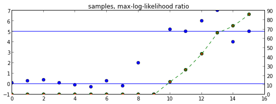
ax = plt.axes()
ax.set_title("samples, max-log-likelihood ratio")
ax.plot(Y, 'o')
ax.axhline(b0)
ax.axhline(b1)
ax2 = ax.twinx()
ax2.plot([log_lhr_max(Y[:T+1]) for T in range(len(Y))], 'go')
ax2.plot([log_lhr_rec(T) for T in range(0,len(Y))], 'r.')
ax2.plot(list(log_lhr_iter(Y)), 'g--')

png