Quantiles
Quantiles and percentiles are an essential tool for the qualitative analysis of telemetry data. In particular, they have become an integral part of performance analysis in the IT domain. Despite their wide use, there are a number of competing definitions of quantiles commonly found in the wild. In this note we will explain how these definitions arise and study their relation in detail. This includes formal relationships, and empirical analysis of practical examples.
Contents
- Quantiles for Random Variables
- Quantiles for Datasets
- Empirical Quantiles
- Quantiles via Sorting
- Practical Choice: The Minimal Quantile for a Dataset
- Interpolated Quantiles
- Interpolated Quantiles from Probability Distributions
- Comparison: Empirical vs. Interpolated Quantiles
- Quantile Implementations
- Conclusion
Quantiles for Random Variables
Let $P$ be a probability distribution on the real axis, and $X$ a $P$-distributed random variable.
Definition. For any number $q \in [0,1]$, a naive q-quantile for $P$ is a number , so that BEGIN_MATH P[X \leq y] = q. END_MATH
Remark.
-
Naive quantiles do not always exist. Take $P=\delta_0$. Here only the numbers 0,1 are realized as naive quantiles.
-
Naive quantile are not always unique. Take $q=.5$ and $P=\half (\delta_0 + \delta_1)$. Here every number $y\in(0,1)$ qualifies as a $.5$-quantile.
To improve the situation, we make the following adjustments to the above definition.
Definition. A number $y$ is a q-quantile, for some number $q \in [0,1]$, and a random variable $X$, if the following conditions are met: BEGIN_MATH P[X < y] \leq q \qtext{and} P[X > y] \leq 1-q END_MATH
Example. If $P=\delta_0$, then
- All numbers $y \leq 0$ qualify as 0 quantile.
- All numbers $y \geq 0$ qualify as 1 quantile.
- All other $0<q<1$-quantiles are $0$.
Example. If $P=\half (\delta_0 + \delta_1)$, then:
- For $0<q<.5$ only $y=0$ is a $q$-quantile.
- For $q=.5$ all numbers $0<y<1$, are $.5$-quantiles.
- For $.5<q<1$ only $y=1$ is a $q$-quantile.
Remark.
- For every $P,q$ there is at least one $q$-quantile.
- As we have seen $q$-quantiles might be non-unique.
- If $X$ has a probability density $p$, which is positive everywhere, then all quantiles are unique.
This definition of Quantile seems to be universally agreed up-on. At least this is what I learned at University (e.g. Georgii - Statistics). and how Wikipedia (accessed on 2019-05-13) defines this. Also I don’t see much room for an alternative definition in this setting.
Quantiles for Datasets
Given a dataset $D=(x_1,…x_n)$ of real numbers, with $n \geq 1$, how can we define quantiles for D?
We will give a few different competing definitions below. But there are a number of undisputed properties, that everyone will find desirable.
Desirable Properties.
- (A) The minimum is a $0$-quantile.
- (B) The maximum is a $1$-quantile.
- (C) The median value is a $.5$ quantile.
- (D) For $D=(x_1 < \dots < x_n), n\geq 2$ the number $x_k$ should be an $\frac{k-1}{n-1}$ quantile.
Special cases of (D) are
- For $D=(0,1,2)$, then $x_2=1$ should be a .5-quantile.
- For $D=(0,1,\dots,10)$, then $x_{10}=9$ should be a .9-quantile.
One natural and very general approach is to assign a probability distribution $P$ to $D$, and then take the quantiles of $P$ as we defined them above. We will follow this strategy in the next sections.
Empirical Quantiles
The simplest probability distribution we can assign to $D$, is the so-called empirical distribution, which looks like this: BEGIN_MATH P_{emp} = \frac{1}{\C D} \sum_{x \in D} \delta_x = \frac{1}{n} \sum_{i=1}^n \delta_{x_i} END_MATH
So a random variable $X_{emp} \sim P_{emp}$ takes values that are uniformly randomly chosen from $D$.
Definition. An empirical $q$-quantile for D is a $q$-quantile of $P_{emp}$. This means, that the following conditions should be met: BEGIN_MATH \frac{\CSet{x \in D}{x < y}}{\C D} \leq q \qtext{and} \frac{\CSet{x \in D}{x > y}}{\C D} \leq 1-q. END_MATH
Remark. Since empirical quantiles are quantiles of a probability distribution, empirical quantiles always exists but are potentially non-unique.
Proposition. Empirical quantile satisfy desirable properties (A)-(F).
Proof.
-
(A) For $y=max(D),q=1$, we have BEGIN_MATH \begin{align} \CSet{x \in D}{x < y} &\leq n-1 \leq n q \nl \CSet{x \in D}{x > y} &= 0 \leq n (1-q). \end{align} END_MATH
-
(B) For $y=min(D),q=0$, we have BEGIN_MATH \begin{align} \CSet{x \in D}{x < y} &= 0 \leq n q \nl \CSet{x \in D}{x < y} &\leq n-1 \leq n. \end{align} END_MATH
-
(C) For $y=median(D), q=.5$, we have BEGIN_MATH \begin{align} \CSet{x \in D}{x < y} &\leq n/2 = q n \nl \CSet{x \in D}{x > y} &\leq n/2 = (1-q) n. \end{align} END_MATH
-
(D) For $D=(x_1,…,x_n)$, $y=x_k$, $q=k/(n-1)$, we have: BEGIN_MATH \begin{align} \CSet{x \in D}{x < x_k} &= k-1 \leq \frac{n}{n-1} (k-1) = q n \nl \CSet{x \in D}{x > x_k} &= n-k \leq \frac{n}{n-1} (n-k) = (1-q) n. \end{align} END_MATH
QED.
Comment. I always assumed that this was the only sensible quantile definition for datasets, that should be used. Hence, this is what I used in my Statistics for Engineers courses. As we will see, there are competing views on this.
Quantiles via Sorting
Quantiles of datasets are commonly computed by sorting the dataset.
Let BEGIN_MATH D_{sorted} = (x_{(1)} \leq x_{(2)} \leq \dots \leq x_{(n)}) END_MATH be the sorted version of $D$. As a convention we set $x_{(i)}=-\infty$ for $i \leq 0$ and $x_{(i)} = \infty$ for $i > n$.
In order to simplify the arguments below we introduce the following notation: BEGIN_MATH \begin{align} Count_{<}(D; y) &= \CSet{ x \in D }{ x < y } \quad & \quad Count_{\leq}(D; y) &= \CSet{ x \in D }{ x \leq y } \nl Count_{>}(D; y) &= \CSet{ x \in D }{ x > y } \quad & \quad Count_{\geq}(D; y) &= \CSet{ x \in D }{ x \geq y } \nl \end{align} END_MATH
Clearly we have:
BEGIN_MATH \begin{gather} Count_{<}(D; y) + Count_{\geq}(D; y) = \C D = n \nl Count_{\leq}(D; y) + Count_{>}(D; y) = \C D = n. \end{gather} END_MATH
The following lemma summarizes the relation between counts and the position of $x$ in $D_{sorted}$.
Lemma. For a dataset D and a number $k \in \{1,\dots,n\}$ we have: BEGIN_MATH Count_{<}(D; x_{(k)}) \leq k-1 \qtext{and} Count_{\leq}(D; x_{(k)}) \geq k. END_MATH For any number $y$ and $k \in {1,\dots,n}$ we have: BEGIN_MATH \begin{align} Count_{<}(D; y) \geq k \;\IFF\; x_{(k)} < y, &\quad Count_{\leq}(D; y) \geq k \;\IFF\; x_{(k)} \leq y \nl Count_{<}(D; y) \leq k \;\IFF\; x_{k(+1)} \geq y, &\quad Count_{\leq}(D; y) \leq k \;\IFF\; x_{(k+1)} > y \nl \end{align} END_MATH
Proof. For the first inequalities it suffices to note that, of all numbers in $D$, at most the numbers $x_{(1)},\dots,x_{(k-1)}$ might be smaller than $x_{(k)}$. For the second one, we have at least $k$ numbers $x_{(1)},\dots,x_{(k)}$ which are smaller or equal to $x_{(k)}$.
Now to the next set of inequalities: We have $Count_{<}(D; y) \geq k$ if and only if $x_{(1)},\dots,x_{(k)} < y$, which is the case if and only if $x_{(k)}<y$. Similarly for $Count_{\leq}$.
We have $Count_{<}(D; y) \leq k$ if and only if $Count_{\geq}(D; y) \geq n - k$. This is the case if and only if $x_{(n)},\dots, x_{(n-(n-k)+1)} = x_{(k+1)} \geq y$. Similarly for $Count_{\leq}$. QED.
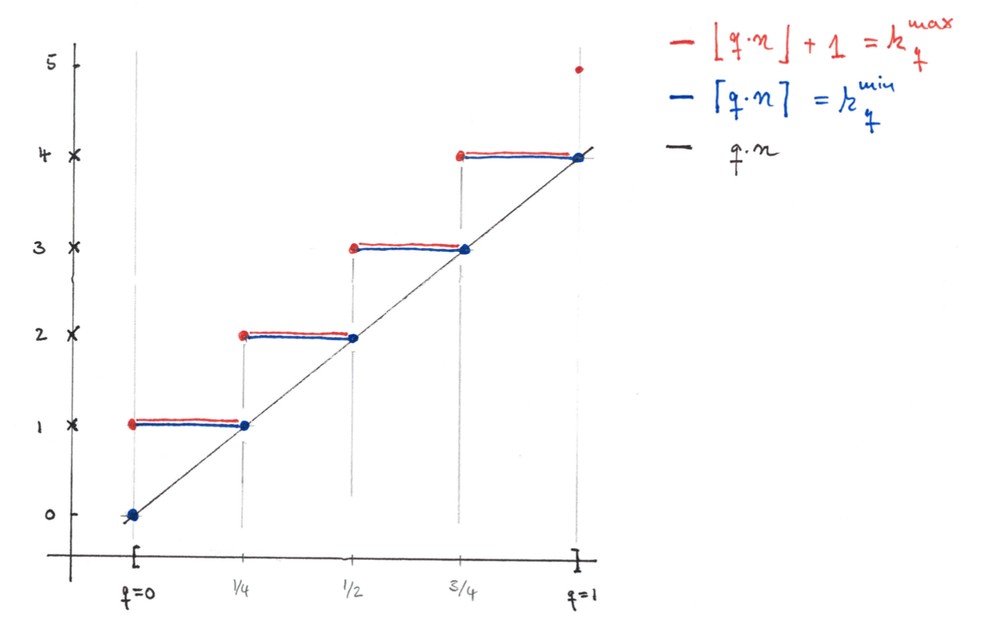
Theorem. The empirical $q$-quantiles are exactly the numbers $x_{(a)} \leq y \leq x_{(b)}$ with BEGIN_MATH a = \ceil{q n} \qtext{and} b = \floor{q n} + 1. END_MATH
Proof. With the above notation, the empirical quantile condition looks like this: BEGIN_MATH Count_{<}(D; y) \leq q n \qtext{and} Count_{>}(D; y) \leq (1-q) n. END_MATH
Lets assume $Count_<(D; y) \leq n q$. Since $Count_<(D; y)$ is an integer, this condition is equivalent to $Count_<(D; y) \leq \floor{n q} = b-1$. By the last lemma we know that his is the case if and only if $y \leq x_{(b)}$.
Similarly, let’s assume $Count_{>}(D; y) \leq (1-q) n$. Subtracting form $n$ on both side, this is equivalent to $Count_\leq(D; y) \geq n q$. Since $Count_\leq(D; y)$ is an integer, this condition is equivalent to $Count_<(D; y) \geq \ceil{n q} = a$. By the last lemma we know that this is the case if and only if $y \geq x_{(a)}$.
QED.
In the light of the theorem, we make the following definition.
Definition. For any number $n$ and $0 \leq q \leq 1$ we define the quantile indices
And for a dataset $D$ of length $n$ we define the minimal and maximal empirical $q$-quantiles as:
where $x_{(k)}$ is the k-th entry in $D_{sorted}$.
Furthermore, we call
the central empirical $q$-quantile.
Example. For $n=1, D=(x)$we have the following quantiles:
| $q$ | $k^{min}_q$ | $k^{max}_q$ | $\QEMIN{q}$ | $\QEMAX{q}$ | Comment |
|---|---|---|---|---|---|
| 0 | 0 | 1 | $-\infty$ | $x$ | Every number $y \leq x$ is a 0-quantile |
| $0<q<1$ | 1 | 1 | $x$ | $x$ | Only $y=0$ is a $q$-quantile |
| 1 | 1 | 2 | $x$ | $\infty$ | Every number $y \geq x$ is a 1-quantile |
Example. For $n=2, D=(x_1 \leq x_2)$ we have:
| $q$ | $qn$ | $k^{min}_q$ | $k^{max}_q$ | Comment |
|---|---|---|---|---|
| 0 | 0 | 0 | 1 | Every number $y \leq x_1$ is a 0-quantile |
| $0<q<1/2$ | 0 < $qn$ < 1 | 1 | 1 | Only $y=x_1$ is a $q$-quantile |
| $1/2$ | 1 | 1 | 2 | Every $x_1 \leq y \leq x_2$ is a $1/2$-quantile |
| $1/2<q<1$ | 1 < $qn$ < 2 | 2 | 2 | Only $y=x_2$ is a $q$-quantile |
| 1 | 2 | 2 | 3 | Every number $y \geq x_2$ is a 1-quantile |
Example. For $n=4, D=(x_1\leq \dots \leq x_4)$ we have:
| $q$ | $qn$ | $k^{min}_q$ | $k^{max}_q$ | Comment |
|---|---|---|---|---|
| 0 | 0 | 0 | 1 | Every number $y \leq x_1$ is a 0-quantile |
| $0<q<1/4$ | 0 < $qn$ < 1 | 1 | 1 | Only $y=x_1$ is a $q$-quantile |
| $1/4$ | 1 | 1 | 2 | Every $x_1 \leq y \leq x_2$ is a $1/4$-quantile |
| $1/4<q<1/2$ | 1 < $qn$ < 2 | 2 | 2 | Only $y=x_2$ is a $q$-quantile |
| $1/2$ | 2 | 2 | 3 | Every $x_2 \leq y \leq x_3$ is a $1/2$-quantile |
| $1/2<q<3/4$ | 2 < $qn$ < 3 | 3 | 3 | Only $y=x_3$ is a $q$-quantile |
| $3/4$ | 3 | 3 | 4 | Every $x_3 \leq y \leq x_4$ is a $3/4$-quantile |
| $3/4<q<1$ | 3 < $qn$ < 4 | 4 | 4 | Only $y=x_4$ is a $q$-quantile |
| 1 | 4 | 4 | 5 | Every number $y \geq x_4$ is a 1-quantile |
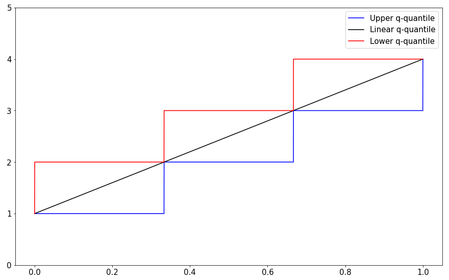
The following figure illustrates the quantile locations for $n=4$.
Comment. A frequently cited source for practical quantile computation is [Hyndman-Fan 1996]. This paper contains a list of 9 different types of quantile definitions that are found in the wild. The minimal empirical quantile $\QEMIN{q}$ is the very fist in their list (Type 1):
Definition 1. The oldest and most studied definition is the inverse of the empirical distribution function obtained by … For this definition $Freq(X_k < Q_1(P)) = \ceil{pn}$
The central empirical quantile $\QE{q}$ is the second entry in their list (Type 2):
Definition 2. $Q_2(p)$ is similar to $Q_1(p)$except that averaging is used when $g=0$…
This underlines the practical relevance of the empirical quantiles.
Practical Choice: The Minimal Quantile for a Dataset
In practical applications one often want’s to make statements of the form:
95% of all requests were served within 500ms.
The quantile version that allows you to make those statements exactly, is the minimal empirical quantile.
Proposition. For a dataset $D$, the following statements are equivalent:
-
p% of all samples in $D$ were less or equal to y.
-
The the minimal p/100 quantile, was greater or equal to y: $\QEMIN{p/100} \geq y$.
Proof. We have seen in the proof of the last theorem, that the condition $Count_\leq(D; y) \geq n q$ is equivalent to $y \geq \QEMIN{q}$. QED.
Comment. This proposition shows, that the empirical quantiles give precise answers to practical questions that arise in the formulation of latency SLAs/SLOs (cf. blog).
Interpolated Quantiles
We already mentioned, that for any definition of quantile we want that $x_{(1)}=min(D)$ should be a $0$-quantile, and $max(D)=x_{(n)}$ should be a $1$-quantile. It’s tempting to define the remaining quantiles by interpolation.
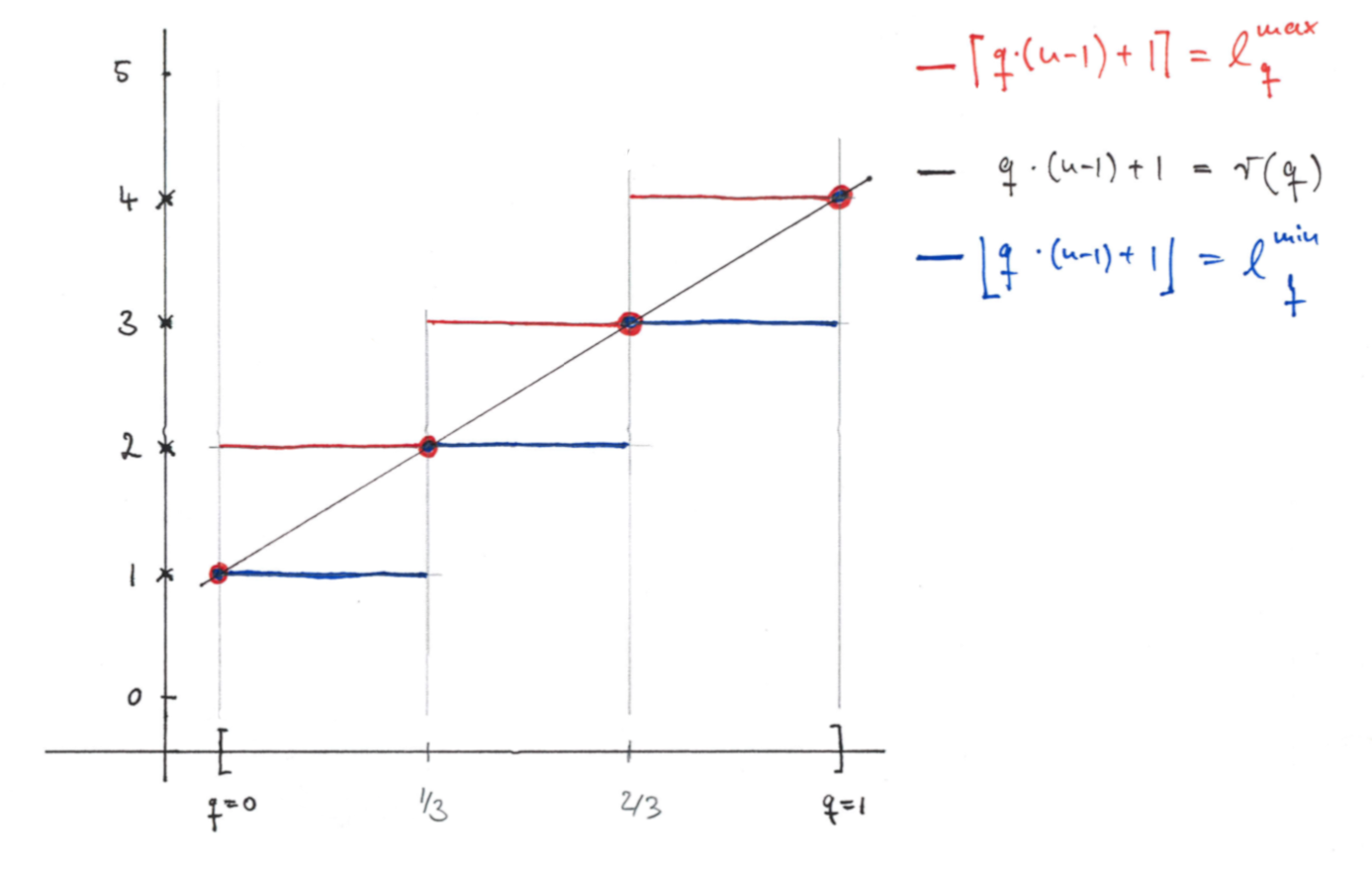
The unique linear function $r$ that interpolates between these cases $r(0)=0$ and $r(1)=1$ is $r(q)= q (n-1) + 1$. Hence it’s natural to consider the following indices:
BEGIN_MATH l^{min}_q = \floor{r(q)}= \floor{q(n-1)} + 1 \quad\text{and}\quad l^{max}_q = \ceil{r(q)} = \ceil{q (n-1)} + 1. END_MATH
Definition. For a dataset $D$ of size $n\geq 2$ and a number $0\leq q \leq 1$ we define the interpolated quantile as:
where $\gamma = q(n-1) - \floor{q(n-1)}$ with $0 \leq \gamma < 1$. Furthermore we introduce the notation
for the minimal and maximal interpolated $q$-quantiles.
Proposition. The interpolated $q$-quantile $\QI$ is a continuous, piece-wise linear function in $q$, with break point at $q=(k-1)/(n-1)$ at which the following values are assumed:
Proof. We have $\gamma=0$ precisely at the break-points $q=(k-1)/(n-1)$ for $k=1,n$.
So if $q=(k-1)/(n-1)$, then
And if $q=(k-1)/(n-1) + \gamma/(n-1)$, with $0 < \gamma < 1$, then $\gamma(q) = q(n-1) - k + 1$ and $l^{min}=k$ $l^{max}=k+1$. So
is a linear function in $q$. Note that for $\gamma=0$ and $\gamma=1$ this agrees with the formula for the break-points. QED.
Example. For $D=(1,\dots,n)$ the interpolated $q$-quantile is exactly $\QI = r(q) = q(n-1) + 1$.
Proposition. The interpolated quantile satisfies the desirable properties (A) - (D) from above.
Proof. (A-C) are direct calculations. We have just proved (D). QED.
Example For $n=4$ the interpolated quantile ranges are at the following positions:
| $q$ | $r(q)$ | $l^{min}_q$ | $l^{max}_q$ | Comment |
|---|---|---|---|---|
| 0 | 1 | 1 | 1 | Only $y \leq x_1$ is a 0-quantile |
| $0<q<1/3$ | 1 < $r$ < 2 | 1 | 2 | The $q$-quantile lies between $x_{1},x_{2}$ |
| $1/3$ | 2 | 2 | 2 | Only $y \leq x_2$ is a 1/3-quantile |
| $1/3<q<1/3$ | 2 < $r$ < 3 | 2 | 3 | The $q$-quantile lies between $x_{2},x_{3}$ |
| $2/3$ | 3 | 3 | 3 | Only $y \leq x_3$ is a 2/3-quantile |
| $2/3<q<1$ | 3 < $r$ < 4 | 3 | 4 | The $q$-quantile lies between $x_{3},x_{4}$ |
| $1$ | 4 | 4 | 4 | Only $y \leq x_4$ is a 1-quantile |
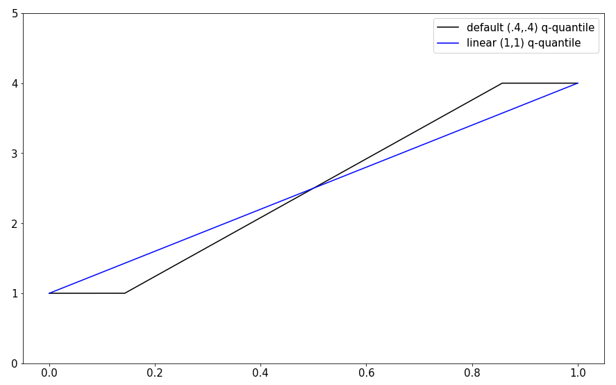
The following figure illustrates the interpolated quantile ranks for $n=4$.
Comment. The Hyndman-Fan list includes our interpolated quantiles as Type 7 quantiles, and attributes them to Gumbel “La Probabilite des Hypotheses” from 1939.
Interpolated Quantiles from Probability Distributions
It is possible to construct a probability distribution that has $\QI$ as associated $q$-quantile. To simplify the discussion, we limit ourselves to the case that $x_{(1)} < \dots < x_{(n)}$ here.
Roughly speaking, we need to construct a probability density function, that spreads the weight of $x_{(k)}$ evenly, across the space between the next higher and next lower samples. One way to do so is to consider the following probability density functions
for which are supported on $[x_{(k)}, x_{(k+1)})$ and integrates to 1.
For each central sample $x_{(2)} \leq x_{(k)} \leq x_{(n-1)}$ we associate $\half (p_{k-1} + p_{k})$. The boundary samples $x_{(1)}, x_{(n)}$ only get a half-weight density $\half p_1, \half p_{n-1}$ respectively. Summing up we get a probability density function:
Proposition. The cumulative distribution function associated to p(x)
has the property that:
- $\cdf(x)$ is continuous and piece-wise linear between $x_{(k)}$ and $x_{(k+1)}$.
- $\cdf(x_{(k)}) = (k-1)/(n-1)$.
Proof. Ad 1) We know that $\frac{d}{dx}\cdf(x) = p(x)$ is constant on between $x_{(k)}$ and $x_{(k+1)}$. Hence $\cdf(x)$ is linear on those intervals.
Ad 2) We have $\int_{-\inf}^{x_{(k)}} p_l(t) = 0$ for $k \leq l$, and $\int_{-\inf}^{x_{(k)}} p_l(t) = 1$ for $k \geq l+1$. So
Corollary. The interpolated quantiles are quantiles for the probability distribution with density $p$.
Proof. The composition $f(q) = \cdf(Q_{int}(q))$ is again a continuous, piece-wise linear function. It suffices to show that $f(q)=q$ on the breakpoints of $f$.
The breakpoints of $\QI$ at $q=(k-1)/(n-1)$, $k=1,\dots,n$ map to the breakpoints of $\cdf(x)$ at $x_{(k)}$, Hence the break-points of the composition $f(q)$ are again at $q=(k-1)/(n-1)$. At those points we have:
Now,
QED.
Comparison: Empirical vs. Interpolated Quantiles
The qualitative differences between empirical- and interpolated quantiles can be well observed in the case $n=4$:
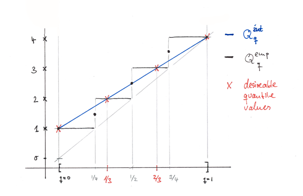
We can see that:
- The interpolated quantiles, take the desirable quantile values at $k/3$ as a basis and interpolate between them.
-
The empirical quantiles, jump at $q=k/4$ to the locations of the samples.
- There are no strict inequalities between the quantile, but for low values of $q$ the interpolated quantile is generally larger than the empirical one. For high values of $q$ the interpolated quantiles are generally lower than the empirical ones.
Also in this example empirical and interpolated quantiles are not far apart. In fact, we have the following proposition.
Proposition. For all numbers $0 \leq q \leq 1$ we have:
Proof. The cases $q=0$ and $q=1$ are trivial. It suffices to show, that for $0<q<1$, we have
We distinguish the cases (A) $q n$ is an integer and (B) $q n$ is not integer.
Case A) Assume $q n$ is an integer. Then $\floor{nq} = \ceil{nq} = qn$. Hence
and
Case B) Assume $q n$ is not an integer. Then $\ceil{q n} = \floor{q n}+1$ and we find:
also, since $qn \leq q(n-1) + 1$ for $0\leq q \leq 1$, we find
QED.
Proposition. Empirical quantile and interpolated quantiles are no more than one sample apart:
Proof. We have seen that the quantile indices satisfy:
So $Q_{emp}(q)$ and $Q_{int}(q)$ both lie within $[x_{(l_q^{min})}, x_{(l_q^{max})}]$. But $|l^{max}_q - l^{min}_q| \leq 1$, hence the difference between the quantiles is bounded by the maximal distance of adjacent samples. QED.
Example. There are cases where interpolated and empirical quantiles are far apart. A common example where this is the case is are long tailed distributions with outliers, and we are interested in high quantiles like $.99,.999$. In these regions samples are sparse and far apart.
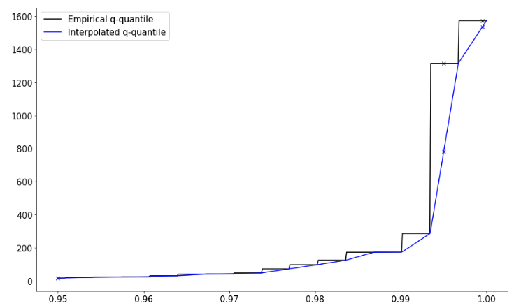
This figure shows data sampled from a Paretro distribution with added outliers like so:
D = [ np.random.pareto(1) for n in range(400) ] +
    [ np.random.pareto(1)*800 for n in range(5) ]
We have marked the following quantile values
| q | Empirical Quantile | Interpolated Quantile | Delta |
|---|---|---|---|
| .95 | 15.920 | 15.927 | 0.007 (0%) |
| .995 | 1386.133 | 793.232 | 592.901 (42%) |
| .9995 | 1623.282 | 1584.152 | 39.13 (2.4%) |
So we see, that the difference between the values can be quite significant in the long tail.
Quantile Implementations
Let’s take a look at how quantiles are implemented in some popular data processing tools.
Numpy
The NumPy function np.percentile, implements interpolated quantiles. As of this writing, there are no options for calculating empirical quantiles with NumPy’s percentile function.
import numpy as np
D = [1,2,3,4]
Q = np.linspace(0,1,5000) # grid
R = np.percentile(D, Q*100,interpolation="linear") # default setting
L = np.percentile(D, Q*100,interpolation="lower")
H = np.percentile(D, Q*100,interpolation="higher")
Scipy
The SciPy function mquantiles implements the continuous quantiles from the Hyndman-Fan list: Type 4-9. This includes the interpolated quantile (Type 7), but not the empirical quantiles (Type 1,2). So, as of this writing, there are no options for calculating empirical quantiles (Type 1,2) with SciPy’s mquantile function.
import numpy as np
from scipy.stats.mstats import mquantiles
D = [1,2,3,4]
Q = np.linspace(0,1,5000)
A = mquantiles(D, Q)
B = mquantiles(D, Q, alphap=1,betap=1) # linear
R
According to the documentation the R quantile function implements quantiles of all 9 Hydman-Fan Types of Quantiles. This includes empirical quantiles (Type 1,2) and interpolated quantiles (Type 4).
The full coverage of the Hydman-Fan list is less surprising, when one takes into account, that Hydman wrote the R quantile function himself:
I wrote a new quantile() function (with Ivan Frohne) which made it into R core v2.0 in October 2004. Everyone computing quantiles in R was now using our code and the paper was cited in the help file. – https://robjhyndman.com/hyndsight/sample-quantiles-20-years-later/
Conclusion
The definition of empirical quantiles is a literal translation of the probabilistic quantiles to the setting of discrete data-sets. The definition of interpolated quantiles is natural form the implementation perspective.
As a sanity check both versions satisfy the desirable properties from our list.
Both quantiles are covered in the encyclopedic Hydman-Fan paper as Types 1,2 and Type 7 respectively. So they can be regarded as well established.
One advantage of the interpolated quantile function is, that is continuous, whereas the empirical quantile function is piece-wise constant with discrete jumps. This property makes the interpolated quantile more suitable for use in plotting applications like the QQ-plot.
One advantage of the empirical quantile is that it gives exact answers to the practical problem of bounding ratios of samples above/below a threshold. This feature makes empirical quantile more suitable for checking SLA/SLO bounds of e.g. latency distributions.
In many cases there is not much of a difference between both versions. When samples are close together, so will be the quantiles in that area. When samples are far apart, like in the long tail of a distribution, the differences can be very substantial.
Apparently most software products prefer to compute interpolated quantiles. Somewhat shockingly for the author, support for empirical quantiles is often entirely lacking, at least in the popular Python libraries.
Summary.
| Property | Empirical Quantile | Interpolated Quantile |
|---|---|---|
| Motivation | Probability Theory | Implementation/Plotting |
| Desirable Properties hold | yes | yes |
| Gives sample ratio bounds | exactly | approximately |
| Continues in q | no | yes |
| Implementation available | not everywhere | widely |
References
- Hyndman, R. J. and Fan, Y. (1996) Sample quantiles in statistical packages, American Statistician 50, 361–365. 10.2307/2684934 robhyndman.com